Few-Shot Text Classification

FF18 · ©2020 Cloudera, Inc. All rights reserved

This is an applied research report by Cloudera Fast Forward. We write reports about emerging technologies. Accompanying each report are working prototypes or code that exhibits the capabilities of the algorithm and offer detailed technical advice on its practical application. Read our full report on few-shot text classification below or download the PDF. You can view and download the code for the accompanying text classification experiments on Github.

Introduction

Text classification is a ubiquitous capability with a wealth of use cases, including sentiment analysis, topic assignment, document identification, article recommendation, and more. While dozens of techniques now exist for this fundamental task, many of them require massive amounts of labeled data in order to prove useful. Collecting annotations for your use case, however, is typically one of the most costly parts of any machine learning application, and demand continues to grow for techniques that make the most of small amounts of data.

At Cloudera Fast Forward, we are no strangers to learning with limited data. We’ve covered multiple techniques in our research, including: active learning, in which humans and machines collaborate to label data in a clever way, essentially bootstrapping from a small amount of labeled data; and meta-learning, in which deep learning algorithms learn to learn.

There are several paradigms for learning from limited amounts of training data. Each of the scenarios outlined below can all be found in machine learning literature—and while definitions continue to evolve, these terms do still tend to have specific meanings.

Few-shot learning for classification is a scenario in which there is a small amount of labeled data for all labels the model is expected to recognize. The goal is for the model to generalize to new unseen examples in the same categories both quickly and effectively.

In traditional zero-shot learning, a classifier is trained on one set of labels and evaluated on a different set of labels that it has never seen before (thus, “zero-shot”). This typically requires providing the model with some type of metadata about the unseen categories in order for it to generalize. (This is the scenario addressed by our meta-learning report, in the context of image classification.) A variation on zero-shot learning is for the model to be evaluated both on never-before-seen and previously-seen labels; this is a more challenging task, because the model must recognize the difference.

Then there’s what we’ll call “on-the-fly” learning. This term is found in ML literature less often. We’ll use it in the context of classification with no training examples at all, and an undetermined number of labels. The goal of the model is to assign examples into some unknown set of possible categories on the fly. This type of model must leverage intrinsic information contained within the labels themselves.

These learning paradigms are agnostic to the types of problems they attempt to solve, and can be found everywhere from computer vision to reinforcement learning. In this report, we’ll focus on text classification, and consider a classic method that can perform under any of these circumstances. Specifically, we’ll concentrate on text embeddings with a modern twist, and demonstrate their versatility as well as their limitations. Finally, we’ll provide insight into best practices for implementing this method.

Latent Text Embeddings

The NLP research team at Hugging Face recently published a blog post that detailed a handful of promising zero-shot text classification methods. We decided to dig a little deeper into one of these methods ourselves. It’s an oldie, but a goodie; we’ll explore how text embeddings can be used for classification.

First, an embedding method is used to generate a document representation and, separately, representations for each of the possible class labels. A document is then assigned the label that lies closest to it in the text embedding space. Note that we do not necessarily need the documents to be labeled a priori (in contrast to supervised learning, in which the model learns relationships explicitly from labeled examples).

This method hinges on the idea that people can categorize documents into named categories without training, because we understand the meaning of the category labels. For example, when reviewing news articles, we can determine whether an article belongs under Science and Technology or Business (or both!) because the words “Science,” “Technology,” and “Business” each have semantic meaning associated with them. The intrinsic meaning of words (in particular, the class labels) is information that we leverage for classification.

Let’s look at an example of how text embeddings can mimic this approach. First, suppose we have a collection of news articles that we’d like to classify into one of the following categories: World News, Business, Science & Technology, or Sports. Next, let’s assume we have a method (the “Embedding Model”) that can assign numeric vectors to text segments. We’ll use the Embedding Model to embed our news article and each of our labels into latent space. (A latent space is simply a compressed representation of the data in which similar data points are closer together).

Suppose this is one of our news articles: “Breaking baseball barriers: Marlins announce first female GM in MLB history.” We’ll pass the text of this article (along with the labels) through our Embedding Model, similar to (though not precisely as) what is shown below.

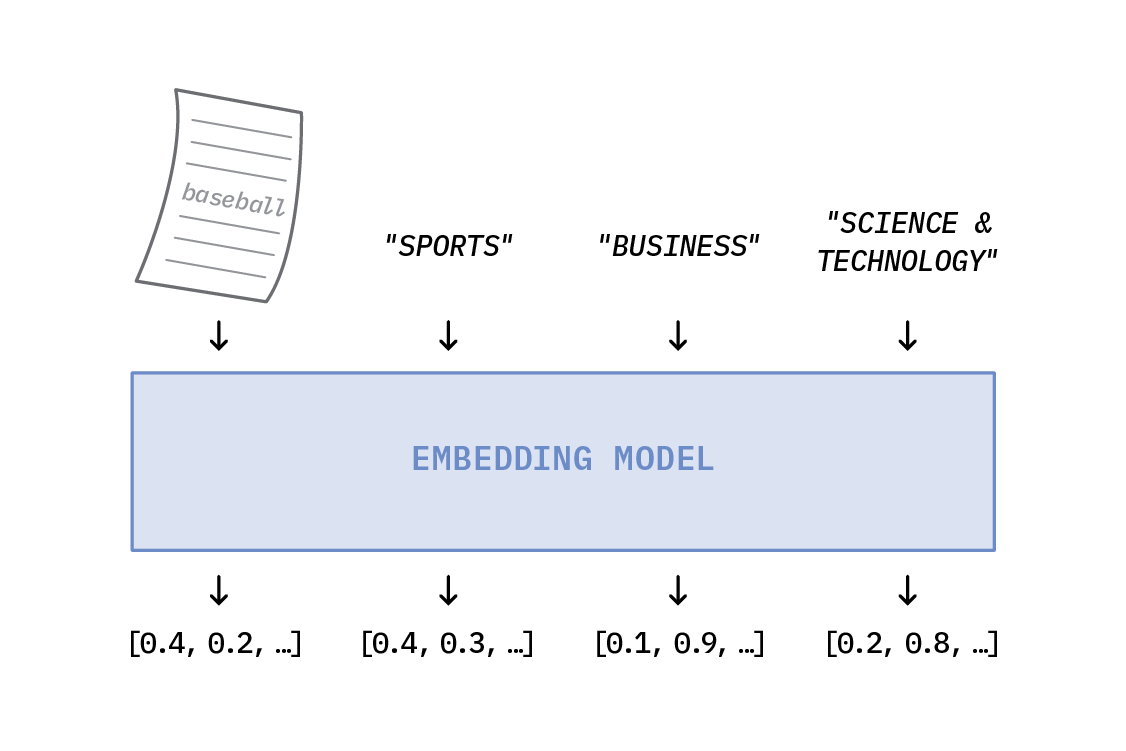
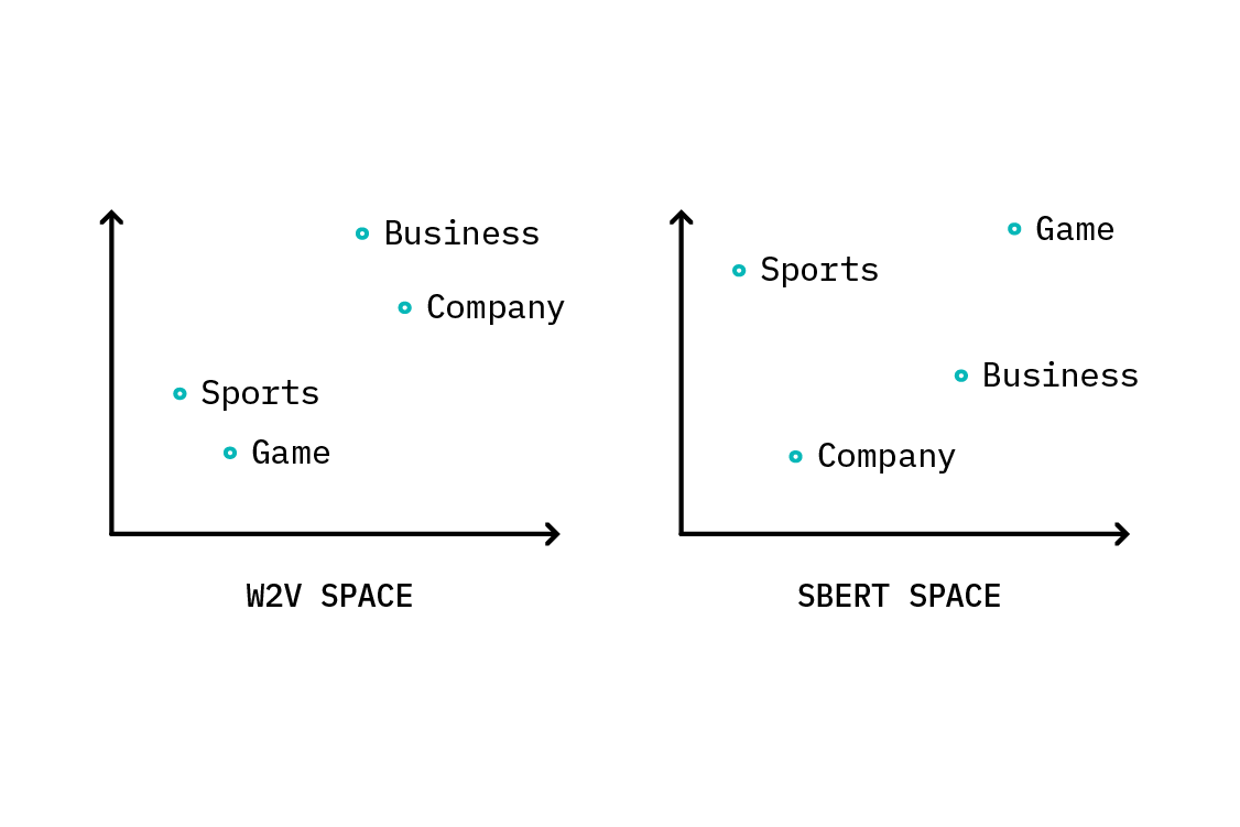
This produces embedding vectors which we can plot in our latent space:

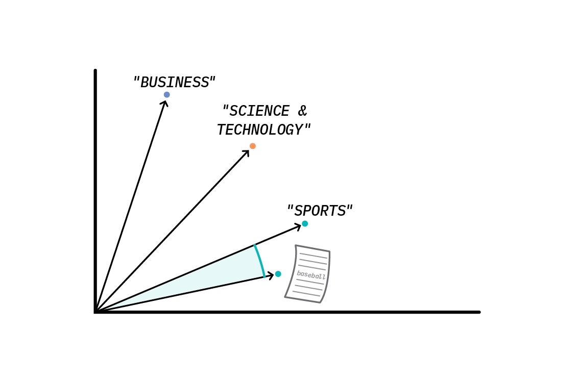
We can now use a similarity metric (like cosine similarity) to compute which of the labels is closest to our news article in latent space, indicating that these text segments are the most similar. In this example, our article is closest to the word “Sports,” so we assign Sports as the label. This is because the word “Sports” is semantically similar to the word “Baseball,” which is the topic of our news article. It was this similarity between words and sentences that allowed us to label the news article—we didn’t use training data at all!

Now, of course, we’ve left a lot out of the discussion. Most pressing: what is this mysterious Embedding Model? And what if we have some labeled examples? And is it really this simple? (Spoiler alert: not quite.) Let’s explore these questions.

The Embedding Model

The latent text embedding method of classification can be implemented with just about any type of text embedding model (and has been—see these examples), though some are definitely better than others! Which embedding model should we choose? In this section, we’ll review some popular approaches, though these are by no means exhaustive.

Representing text numerically is not a new idea, and can be as simple as a bag-of-words or tf-idf vector, or as sophisticated as word2vec or GloVe. Better performance is often achieved from contextual embeddings, like ELMo or BERT, which embed words differently, depending on the other words in the sentence. These approaches focus on words, n-grams, or pieces of words as the basic embedding unit. Deriving a document representation then requires clever aggregation of the word embeddings.

In contrast, sentence embedding methods embed whole sentences or paragraphs; an early example is Doc2Vec, which is similar to word2vec, but additionally learns a vector for the whole paragraph. More recent models include InferSent and Universal Sentence Encoder. Sentence embedding methods obviate the need for ad hoc aggregation techniques, and typically better capture the semantic meaning of whole text segments (as compared to aggregating word embeddings).

Recent advances in sentence embedding methods have prompted us to re-evaluate the latent embedding approach. But first, what about BERT? Isn’t that all the rage these days for everything NLP-related? Shouldn’t we just use BERT to embed our text?

To BERT or not to BERT

Since its inception in 2017, BERT has been a popular embedding model. As we’ll see, however, traditional ways of using BERT for semantic similarity are not ideal for a latent text embedding approach.

BERT outputs an embedding vector for each input token, including word tokens and special tokens, such as SEP (a token that designates “separation” between input texts) and CLS. CLS is shorthand for “classification,” and this token was intended as a way to generate a sentence-level representation for the input. However, experiments have shown that using the CLS token as a sentence-level feature representation drastically underperforms aggregated GloVe embeddings in semantic similarity tests.

Another option is to pool together the individual embedding vectors for each word token; this is the BERT equivalent of pooling word2vec vectors. However, these embeddings are not optimized for similarity, nor can they be expected to capture the semantic meaning of full sentences or paragraphs. While there are plenty of use cases where these embeddings do prove useful, neither is ideal as a latent space for semantic sentence similarity.

Rather than using BERT as an embedding model, we can instead train it to specifically learn semantic similarity between sentences (an example of a sentence-pair regression task): BERT is shown many pairs of sentences, and is tasked with producing a score capturing their similarity. This procedure produces a fantastic semantic similarity classifier, but it is not efficient. In this scheme, BERT can only compare two text segments at a time. If we want to find the closest pair among many, we’ll have to pass every possible sentence pair through the model. Since BERT isn’t known for its speed, this procedure could take a while!

Sentence-BERT (SBERT) addresses these issues. First published in 2019, this version of BERT is specifically designed for tasks like semantic similarity search and clustering—tasks that typically rely on cosine similarity to find documents that are alike. SBERT adds a pooling operation to the output of BERT to derive fixed sentence embeddings, followed by fine-tuning with a triplet network, in order to produce embeddings with semantically meaningful relationships. The result is a model that takes in a list of sentences and outputs a list of semantically salient sentence embeddings, one for each input sentence. These embeddings can be passed directly to cosine similarity, and the closest pair can quickly be determined. The authors demonstrate that SBERT sentence embeddings outperform aggregated word2vec embeddings and aggregated BERT embeddings in similarity tasks. Here is a latent space that we can leverage! SBERT (and SRoBERTa) models are publicly available both on the Sentence-BERT website and in the Hugging Face Model Repository.

Improving this approach with Zmap

Let’s take stock of and outline the latent text embedding method. For a document, d (e.g., a news article), we want to predict a label, l, from a set of possible labels. We apply SBERT to our document, d, and to each of the l labels, treating each label as a “sentence.” We then compute the cosine similarity between the document embedding and each of the label embeddings. We assign the label that maximizes the cosine similarity with the document embedding, indicating that these embeddings are most similar in SBERT latent space. This process can be succinctly expressed as:

We then repeat this for every document in our collection, and voilà!

This actually works relatively well, depending (of course) on the dataset, and the quality and number of labels. But Sentence-BERT has been optimized… well, for sentences! It’s reasonable to suspect that SBERT’s representations of single words or short phrases like “Business” or “Science & Technology” won’t be as semantically relevant as representations derived from a word-level method, like word2vec or GloVe. This means, for example, that the word2vec representation of “Business” could well have a more meaningful relationship with other words in the word2vec latent space than its SBERT representation in SBERT latent space.

In a perfect world, we’d use SBERT to embed our documents, and w2v or GloVe to embed our class labels. Unfortunately, these embedding spaces do not have any inherent relationship between them, so we would have no way to know which labels were closest to our document. We could learn a relationship between these two spaces, but in order to do that, we’d need some annotated data—which defeats the purpose of zero-shot learning!

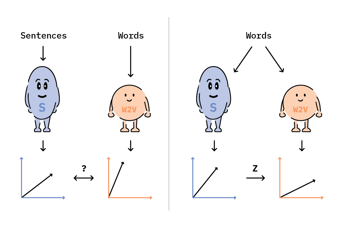
Instead, we can generate an approximation, by learning a mapping between individual words in SBERT space to those same words in w2v space. We begin by selecting a large vocabulary of words (we’ll come back to this) and obtaining both SBERT and w2v representations for each one. Next, we’ll perform a least-squares linear regression with l2 regularization between the SBERT representations and the w2v representations.^[1]

This results in a matrix, Z, which maps SBERT space to w2v space. We’ll use Z to transform both SBERT document representations (e.g., sentences) and SBERT label representations (e.g., words) into a new, lower-dimensional latent space, and perform our cosine similarity classification procedure in this new space.

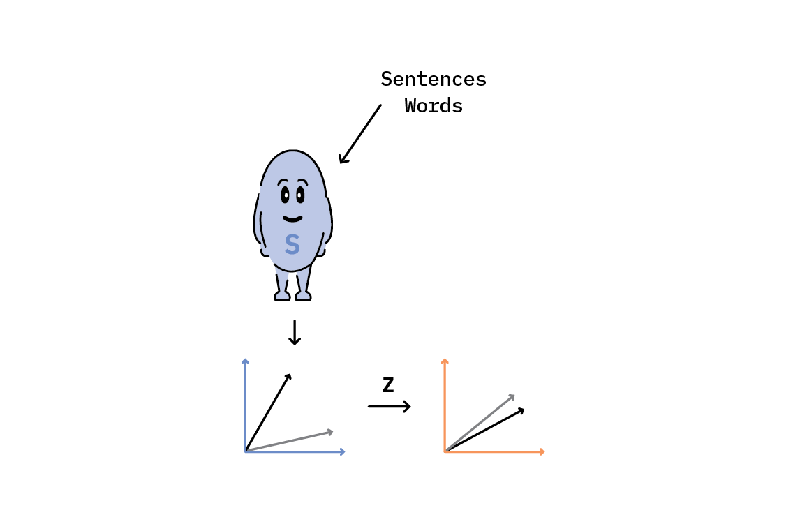
This is how our classification model looks now:

All we’ve done is multiply Z to both the document representation and the label representations, and then maximize the cosine similarity over the label set, as before.

So where does this “large vocabulary of words” come from? One approach (used by the Hugging Face team) is to leverage the fact that w2v (and other popular open-source word embeddings) is trained on a massive corpus of text. Most publicly released word representations are ordered by word frequency, with the most common words at the “top” and rare words at the “bottom.” This means that you can quickly identify a large vocabulary of the most frequently used words in that corpus.

The assumption here is that learning a mapping between SBERT and w2v for the most commonly used words (as measured over a massive corpus of text) will provide a good mapping between the two latent spaces. Another approach we tried is to use the most frequent words in the corpus you wish to classify. In either case, the greatest benefit to both these approaches is that neither requires any annotated data—but each comes with pros and cons. (We’ll discuss those and explore the performance results in the Experiments section below.)

Incorporating labeled data

Everything we’ve discussed so far has been under the premise that we have no labeled data whatsoever (“on-the-fly” learning). But what if you have some? The latent embedding approach is highly adaptable and can be modified to work with annotated examples in each category (few-shot learning), or when we might only have annotated examples for a subset of categories we’re interested in (traditional zero-shot learning). How do we take advantage of these labeled examples? We’ll follow the approach that the Hugging Face team outlines in their blog post, while hopefully providing a bit more context.

This method involves learning another mapping, this time between the documents and their labels—but we need to be careful not to overfit to our few annotated examples. Our goal is to learn a transformation that will rely on the semantic richness of our representations so far (i.e., multiplying SBERT embeddings by Z), while still allowing us to incorporate information from the labeled examples.

One way to accomplish this is to modify the regularization term in the linear regression. Before looking at this modification, let’s take a closer look at the traditional objective function for least-squares with l2 regularization in order to get a feel for how this is accomplished.

Weights, W, are learned through minimizing the loss function, as expressed below:

The first term essentially tells W how to match an input, X, to an output, Y. The second term effectively minimizes the norm of the weights. The result is a set of regularized weights that map X to Y (which was exactly what we wanted in the previous section). Now we’ll modify the regularization term:

The first term still tells W how to map X to Y, but in the second term, the elements of the weight matrix are now pushed towards the identity matrix.^[2]

If we only have very few examples, W will likely be quite close to the identity matrix. This means that when we apply W to our representations, SBERT(d)ZW will be very close to SBERT(d)Z. This is exactly what we want: to rely strongly on our original representations in the face of few examples. If we have many examples to learn from, W will be pushed further away from the identity matrix, in which case it will more strongly modify the composition of SBERT(d)ZW, potentially changing the predicted label for the document, d. Our final classification procedure now looks like this:

It’s important to note that this technique is now akin to supervised learning: W is learned from training examples, and applied to test examples. However, notice that we have not specified whether W is learned in a few-shot way (annotated examples for each relevant label) or in a zero-shot way (annotated examples for only a subset of the labels we are interested in). The approach is the same regardless, which is what makes this technique so flexible.

So how well does it work? Let’s find out.

Experiments

While not comprehensive, this section seeks to provide some background on how different choices in the construction of these mappings affects the outcome of classification. All of our experiments can be found in a collection of Colab notebooks on our github repo.

First, let’s talk data

We explored text classification with two different datasets.

AG News

The original dataset consists of more than one million news articles gathered from more than 2000 news sources by ComeToMyHead (an academic news search engine) in more than one year of activity. We use a subset constructed for topic classification consisting of news articles in four categories. The training set consists of 30,000 articles for each category (120,000 total), while the test set contains 1,900 articles for each category (7,600 total). When performing “on-the-fly” classifications, we used only the test set. We pulled the AG News topic classification dataset from the open-source Datasets repository maintained by Hugging Face.

Reddit

This dataset contains nearly four million preprocessed submissions and comments from Reddit, collected between 2006 and 2016. It restricts to only those posts that include a “TL;DR” summary, which we use as the text we wish to classify into one of many possible subreddits (our target variable). We filtered this dataset down to the top 16 most popular subreddits by number of posts, resulting in over 600,000 examples. We randomly selected a stratified 10% of the posts as a test set, which we used in our “on-the-fly” classification. The full dataset can also be obtained from the Datasets repository maintained by Hugging Face.

Improving on-the-fly classification with Zmap

Earlier, we talked about creating a mapping between SBERT and w2v spaces by comparing where individual words live in each of those spaces. This requires selecting a vocabulary of words. Which words create the best map? And how many words do you need?

How many words do you need?

Bigger isn’t always better. We explored the general effect on classification accuracy of a Zmap constructed from different numbers of words. We built a vocabulary from the most frequent words as measured over the corpus on which word2vec was trained. We first constructed Zmap from the top 100 most frequent words, then the top 200 most frequent words, and so on, until we’d included the top 100,000 most frequent words. With Zmap constructed, we then measured the accuracy of the resulting classification for both the AG News and Reddit datasets. The figure below shows the behavior we observed. As we increased the number of words used to construct Zmap, classification scores also increased, but only to a point. Eventually, after about 20,000 words, scores tended to decrease again. Why?

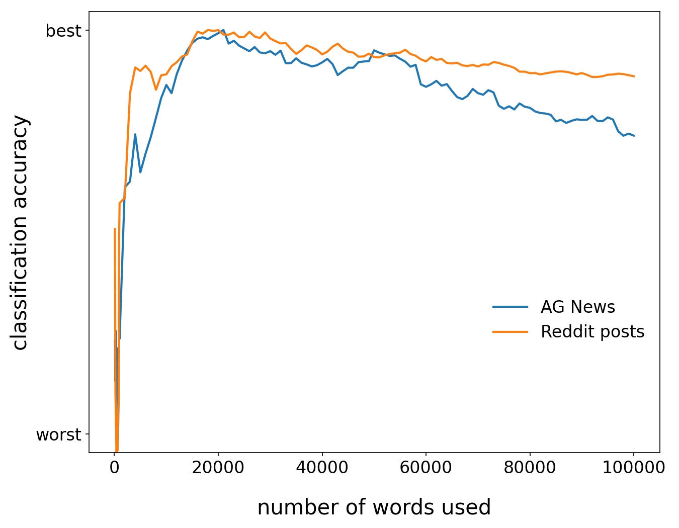
The answer is likely largely due to the fact that we’re including rarer words, which could be interpreted as noise. The words are in descending order by frequency; this means the most common words are at the “top,” so as we include more words, we’re including rarer words.

The matrix, Zmap, is a fixed size because it maps from SBERT space (where embedding vectors are 768 elements long) to w2v space (where embedding vectors are only 300 elements long). This means that Zmap has dimension (768, 300), regardless of how many words are used to construct the mapping. When we have only a few words (say, 100), Zmap doesn’t contain enough information to provide a useful transformation, so the overall classification suffers. When we have 100,000 words, the rare words dilute the effect of the more common words and again, the overall classification suffers.

There seems to be a sweet spot around 20,000 words—a finding we did not expect, but saw echoed in other datasets we tried (but do not show here). This peak is quite broad, and using anywhere from 15,000-25,000 words will likely optimize Zmap. However, using this optimized Zmap does not necessarily result in the best overall text classification. (We’ll explain this cryptic statement in the next section.)

Which words make the best Zmap?

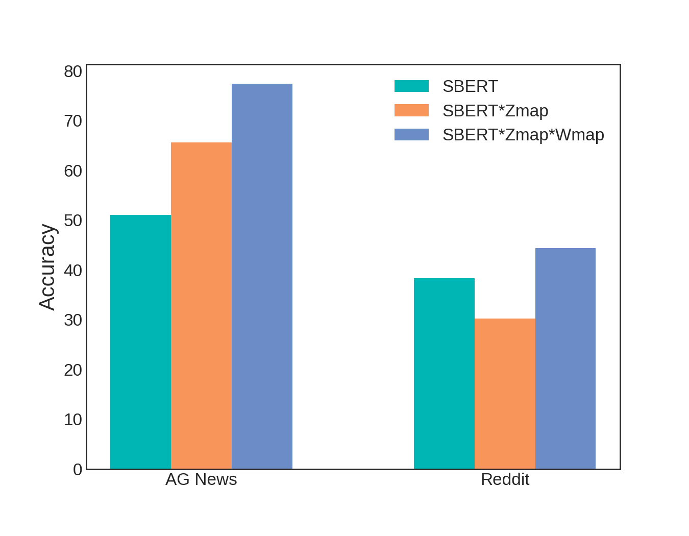
Instead of working in relative terms, let’s get specific, and explore the efficacy of Zmap. Below, we compare the classification accuracy of the latent text embeddings method using only SBERT representations, and transforming those representations with Zmap.

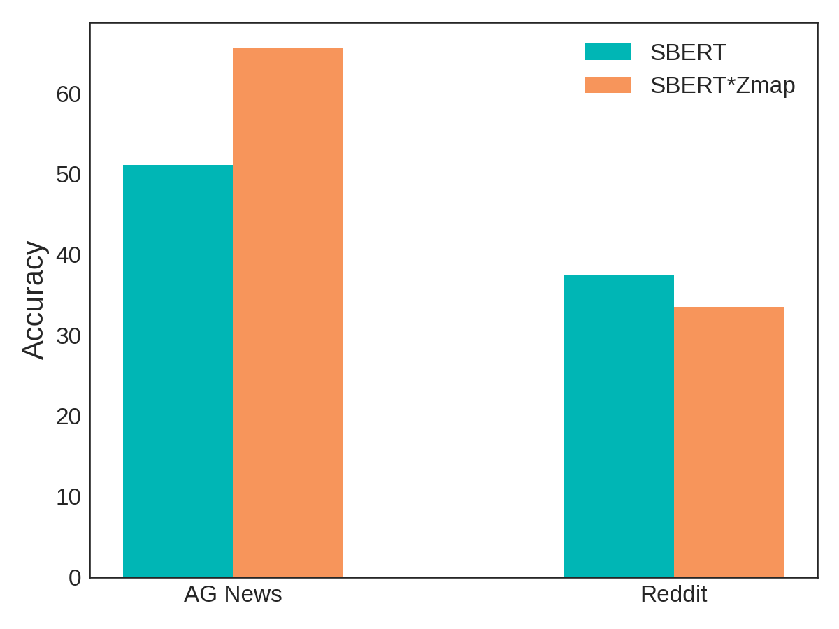
The teal bars represent classification accuracy when using only SBERT representations. We achieve over 50% accuracy for AG News, and nearly 40% accuracy for the Reddit dataset. While these might not seem like numbers to write home about, keep in mind that we did not perform any supervised training procedure! In general, scores are worse for the Reddit dataset because it’s simply harder to correctly classify into ten categories rather than only four. In both cases, scores reflect better-than-random accuracy, so we’re definitely on the right track.

The orange bars illustrate the effect of transforming SBERT representations with a Zmap constructed from a vocabulary of 20,000 words. We observe a dramatic increase in performance for the AG News dataset: nearly 15 points! However, the news isn’t so rosy for the Reddit dataset, where we actually see a drop in classification accuracy. What gives?

To dig a bit deeper, let’s perform some cursory error analysis. Below, we break down the predictions for the AG News dataset by category for both the SBERT-only and SBERT+Zmap classification procedures. Each category contains 1,900 examples, so if our classification were perfect, each bar would fall exactly at 1,900 examples in the diagram below. Looking at the teal bars (SBERT-only), we instead see a plurality of the news articles were predicted under the World category, with only a paltry few predicted as Sports. Once we transform these representations with Zmap (orange bars), we see the predictions begin to balance out between the four categories, which results in that dramatic 15 point accuracy increase.

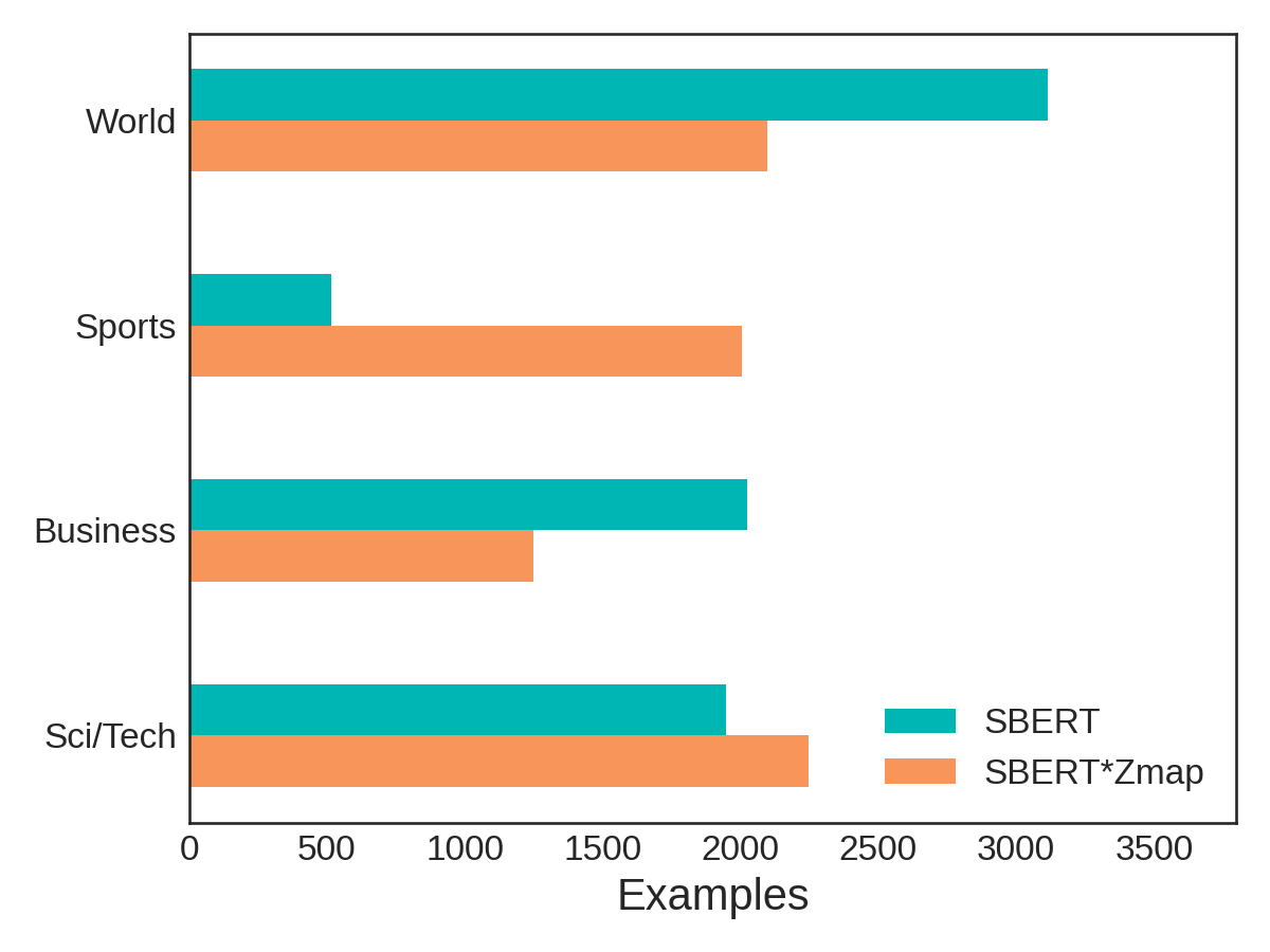
We speculate that the word “World” is so vague and all-encompassing that many news articles would end up being closer to this word than any other category name in SBERT space. Once we have a better mapping between SBERT space and w2v space (which is better at capturing the semantic meaning of individual words), more articles are predicted to be Sports. This is great! And it’s exactly what we expected Zmap to do.

So why didn’t this work for the Reddit dataset? We constructed Zmap from a vocabulary of 20,000 most frequently used words in the corpus on which word2vec was originally trained, which happens to be a large portion of the Google News corpus. Perhaps this is why it performs so well with AG News, but not Reddit—words that are very common in one news corpus (Google News) might provide a better mapping for another news corpus (AG News) than for a collection of user posts and comments on Reddit.

To address this, we constructed a new Zmap from the 20,000 most frequently used words in the Reddit corpus. Below, we break down the predictions for the Reddit dataset as we did previously for the AG News dataset. This time, we show three bars for each category (subreddit name), corresponding to predictions using SBERT only, SBERT transformed with Zmap constructed from w2v words, and SBERT transformed with Zmap constructed from Reddit words. In this case, each category contains 1,300 examples, so if our classification were perfect all the bars would be the same height and fall exactly at 1,300 examples.

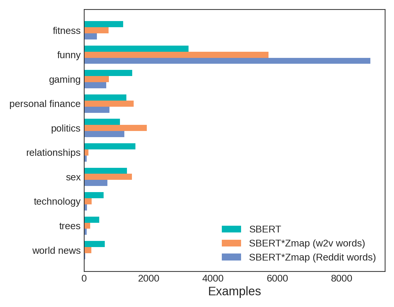
Instead, we see something rather peculiar. Using SBERT representations alone (teal bars), we find posts are predicted under the Funny subreddit more than any other. “Funny” is a pretty general word, much like “World” was in the AG News example. However, this time, applying various Zmaps only serves to exacerbate the discrepancy!

Rather than revealing a flaw in the method, we surmise that this is exactly what we should expect. While both “Funny” and “World” have broad, sweeping meanings, we argue that “Funny” is even more universal. Posts from any of these ten subreddits could easily be considered “Funny,” since humor is a common mode of communication among humans. Whether we’re talking about fitness or finance, we like to laugh!—and when we create better mappings between SBERT sentence space and w2v word space, we’re reinforcing that nearly everything can be funny.

This example serves to highlight a limitation of the latent text embedding method: not only do category labels need to have semantic meaning, they also need to have specific semantic meaning to maximize the method’s utility.

In general, an optimal Zmap will usually provide a better representation for classification. We find that constructing it from a vocabulary of 20,000 words is sufficient, and those words can come either from the w2v corpus, or from your own corpus. This technique is entirely unsupervised (as these words come either from open sources or from your own data), and it requires zero annotated examples.

So far, our experiments have focused on the performance of the latent text embedding method that does not rely on any labeled data whatsoever. Let’s now turn to another, perhaps more likely scenario: having some labeled data, but perhaps not enough to rely on traditional supervised classification techniques.

Few-shot classification by optimizing Wmap

We’ll start by assuming that our SBERT representations transformed by Zmap provide a good starting point for classification in latent space. We’ll then use labeled data to learn an additional mapping, Wmap, between example representations and their corresponding label representations. Wmap will then be applied as a second transformation before classification.

In general, Wmap provides a nice boost in classification accuracy on both the AG News and Reddit datasets, as shown below. In this figure, the blue bars represent measured accuracy after training on 500 AG News and 30 Reddit examples in each of their respective categories. This amounts to a total of 2,000 training examples for the AG News dataset, and 300 training examples in the Reddit dataset. Should we have used more labeled examples? Could we get away with fewer?

It turns out that not only is this method great for limited amounts of labeled data, it can only handle limited amounts of labeled data! We explored how accuracy changed as a function of training on an increasing number of annotated examples. Known as learning curves, these figures are a quick way to assess the general performance of your model, as well as possible areas of overfitting.

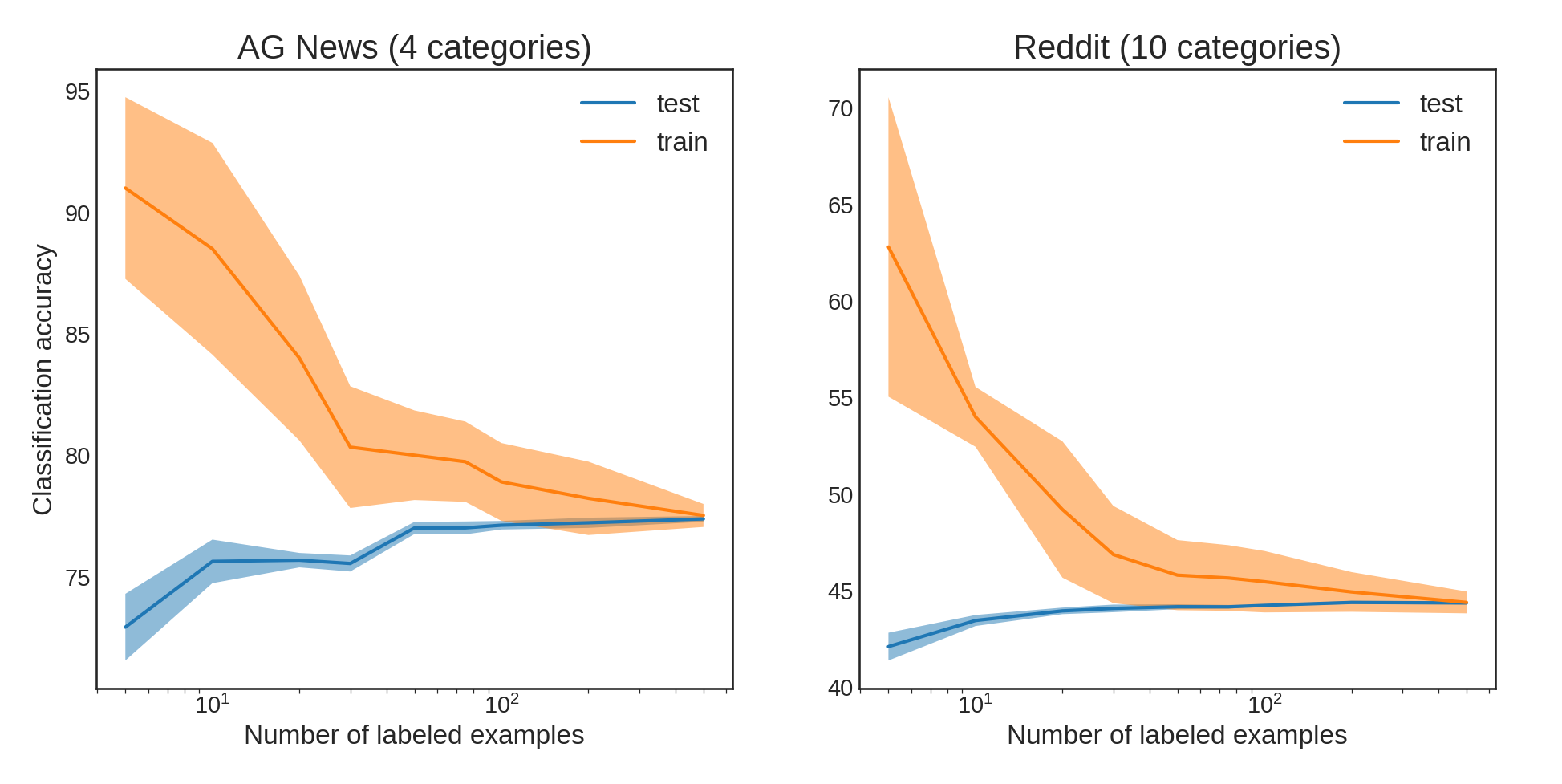
In both cases, training with very few examples is likely to lead to overfitting, in which the model essentially memorizes the training set, and thus does not generalize well to the test set. This happens even with a significant amount of regularization when training Wmap. However, we see this effect is mitigated when training on around 100 examples per category. The test accuracy plateaus quickly, which means that training on additional examples is unlikely to provide any further increase in accuracy.

To answer our earlier questions: for the AG News dataset, we probably didn’t need 500 examples per category; 100 each would have yielded similar results. For the Reddit dataset, 30 examples per category probably resulted in a slightly overfit Wmap. We would be better served if we doubled the number of training examples in each category.

It might seem disappointing that these scores plateau so quickly, and that it’s essentially useless to train on more than about 100 examples per category, but keep in mind that generalization in machine learning stems largely from the ability of the model to capture increasingly complex statistical patterns. This is typically only possible with larger models, i.e., more parameters. In our case, Wmap is a fixed size, and thus it is quickly saturated—which is why more training examples do not provide additional gains. But this is great news for learning with limited data; not only does the method work well in this regime, it’s actually perfectly suited! If you find yourself with more than a couple hundred labeled examples in each of your categories, you will likely be better off exploring a more traditional ML approach that can better capture the data’s complexity.

Interpretability

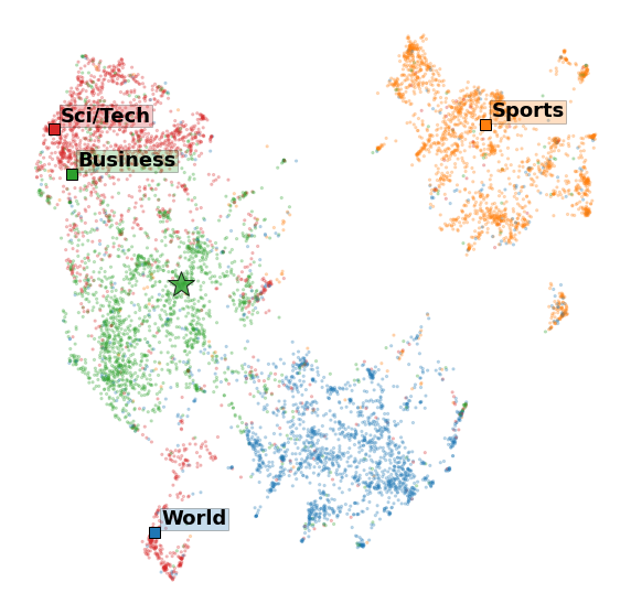
Another benefit of the latent text embedding method is its inherent interpretability. Word2vec has been lauded for its interpretability, with the discovery that the numerical representations of words could be added and subtracted—the result of which would be the numerical representation of a word that completes an analogy. For example, the expression “Paris” + “France” - “Italy” would yield an embedding vector that is very close to the word “Rome.” While it’s unclear if SBERT space operates similarly to w2v space (and what does it even mean to add and subtract documents?), having all the documents and labels embedded into the same latent space provides us with insight into why documents are predicted to have a given label.

In the figure below, we embedded the AG News test set and the four category names (using SBERTZmap) and used the UMAP algorithm to render a two-dimensional embedding that we could visualize. We see that, in general, most articles cluster well around or near their label. The star represents a specific article that was predicted to have the label Business, and we can see that it is, in fact, closest to the label Business. This is the inherent power of latent embedding spaces for interpretability.

Limitations

While the latent text embedding approach provides a flexible and semi-interpretable way to classify text, it’s not without its limitations.

Validation is a challenge

Let’s address the elephant in the room: we had access to labeled training and test sets for all the experiments performed for this report, which is how we were able to assess the performance of Zmap. In a real-world, “on-the-fly,” no-labeled-data-available situation, validating the results of the method is essentially impossible. This is why we spent time looking for possible generalities that could provide guidance on how to use this method in a practical application—but, as we saw with the Reddit dataset, sometimes Zmap actually makes your classification accuracy worse! And without labeled data to validate the method, you will have no way of knowing if this is the case for your data.

This isn’t solely an issue with the latent text embedding approach—this is a challenge for any unsupervised learning situation. The solution, unfortunately, is to simply buckle down and label some data! As we saw, even just a couple hundred examples can provide a wealth of insight and performance gains.

Meaningful labels are a necessity

It’s not enough to have a few labeled examples for training or validation; care must be taken when deciding what the label names themselves will be. This method relies on labels laden with meaning, and that possess some semantic relationship to the text documents you wish to classify. If, for example, your labels were Label1, Label2, and Label3, this method would not work, because those labels are meaningless.

In addition to being meaningful, label names should not be too general. As we saw, the words “World” and “Funny” were too broad and all-encompassing to be practical label names. While an optimal Zmap was able to correct for this effect in the World example, this won’t always be the case, as we saw with the label Funny.

This probably won’t beat supervised methods

Finally, in terms of performance metrics like accuracy or F1 score, the latent text embedding approach won’t beat out standard supervised text classification methods. We saw that even the best optimization of Wmap could only increase the classification accuracy by 10-15 points, and training on more labeled examples didn’t help. If you have a good amount of labeled data, it’s worth checking out traditional supervised approaches first.

Conclusion

Text is everywhere. The amount of text data in the world is rapidly increasing, but much of it is not labeled. Classifying text data is not only a goal in and of itself, but is often a stepping stone to a wealth of more complex capabilities such as recommendation systems and sentiment analysis. This has fueled research to pursue new text classifications techniques that make the most of a few labeled examples. However, classic techniques, like latent text embeddings, should also not be overlooked, especially with the advent of new and improved text embedding algorithms like Sentence-BERT.

While there are limitations to the method, we like the latent text embedding approach because of its simplicity, flexibility, and interpretability. This method is a great starting point for situations in which only a few labeled examples exist. Additionally, this method could serve as a strategy for bootstrapping those few labeled examples into many more—by allowing a human to identify and label articles closest to those which are already annotated, or which are most similar to the label name of interest.

We built a demo of this method that you can try out for yourself. It allows the user to play around with the various strategies presented here—including the application of Zmaps and trained Wmaps—for the AG News dataset. You can spin it up easily by cloning our github repo. Check it out!

---

1. It turns out that the solution to ordinary least squares with l2 regularization can be written as a concise equation, so we do not need to perform gradient descent to learn the weights. Instead, we need only invert a matrix. For intuition on how to interpret least squares as a linear algebra problem, check out this fantastic blog post. ↩︎

2. As the Hugging Face team points out, this is equivalent to Bayesian linear regression with a Gaussian prior on the weights, centered at the identity matrix. Our prior belief is that our embedding mechanism, SBERT(d)Z, produces good text representations, and we only update this belief (move away from the identity matrix) as we see more training examples. ↩︎